Contrastive Deep Explanations
[Explainable AI Deep Learning 1. Introduction
As the creation of large deep learning models has advanced, researchers have become curious about what happens inside these models. Even though many people use these models in their daily basis like grammar checking, self-driving cars, weather prediction, or more specialized areas such as cancer detection or predicting a protein’s 3D structure from its amino acid sequence, etc., nobody really knows how these models work internally. In cases where deep learning is used on medicine or self-driving cars, it is particularly important to know the reasoning behind the model’s decisions—for example, understanding why did not the model chose prediction B over the prediction A.
Note: I will interchangeably use model or a neural network.
In this article, I will explain the paper CDeepEx: Contrastive Deep Explanations, which introduces a method capable of answer the question of Why did you not choose answer B over A and provided an overview of the concepts that a network learn.
Figure 1: This is an example of a classifier trained on the MNIST dataset. Its input is an image of a handwritten digit, for example the number 3 and the model predicts this number with a confidence of 72%. The paper address the question of Why the classifier predicts the number 3 instead of the number 9 by showing how the image 3 can be transformed to make the classifier predict this new image as the number 9.
2. CDeepEx: Contrastive Deep Explanations
To archive contrastive explanation i.e., to answer Why did you not choose answer B over A, the proposed method uses a generative latent-space model. This involves using a Wasserstein Generative Adversarial Networks (WGAN) or Variational AutoEncoder (VAE). The models learn a latent-space of the data, where is captures the fundamental information that compose the data. The latent-space can be viewed as a bridge between the network and human understanding of the data. The idea is to use a WGAN or VAE to learn this latent-space for later than be used to generate images that can explain a model’s reasoning process.
Figure 2: These are two generative models. (a) is a variational Autoencoder (VAE), where an image is inputted on the encoder, and using a code, it generates a latent representation where the input (image) is transformed into a lower- dimension that preserves the essential information of the input. The decoder uses this latent representation to reconstruct an image that is similar to the input. (b) Is a Wasserstein GAN (WGAN) where random noise is used to generate images that look similar from the data, and a discrimination is used to predict how real an image it is.
Note: The latent representation is simply a point in the latent space. Remember that the goal of the WGAN or VAE is to create this latent space which contains the information the model learn from the data.
The code (for VAE) and the random noise (for WGAN) can be viewed as the latent space. Since both the code and the random noise comes from a normal distribution is possible to sample a point from normal distribution and inputted in the decoder (for the VAE) and the generator (for the WGAN) to generate an image. The only component used to generate the explications is the decoder in the VAE and the generator in the WGAN.
To generate explication is use a generator (a network that generate natural images) and the discriminator (the classifier of interest). The image $\mathcal{I}$ is inputted into the discriminator network $D$ to produce $y_{true}$. The class label of interest will be denoted as $y_{probe}$. Thus, we can formulate the question of Why did $D$ produce label $y_{true}$ and not label $y_{probe}$ for the input $\mathcal{I}$?.
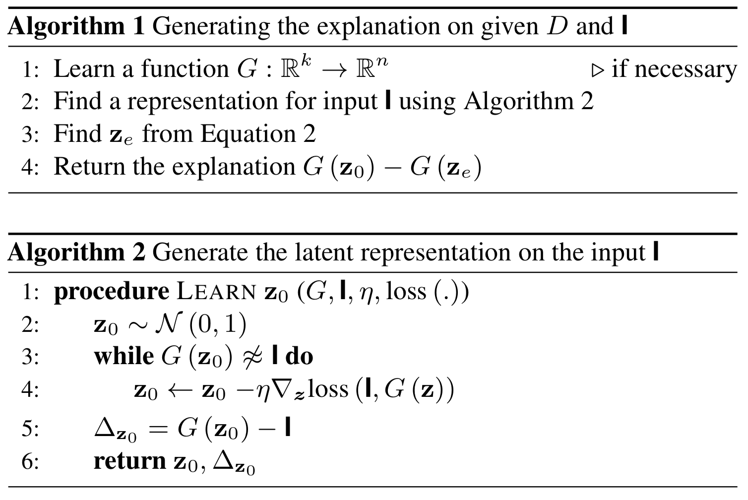
To generate explanation:

In these algorithms, the first step is to train a generator $G$ that, given a latent representation of real values of size $k$, outputs an image of size $n$. After training the generator, we need to find a representation $z_0$ that, when inputted to $G$ generates an image similar to $\mathcal{I}$. Initially, $z_0$ is sampled from a normal distribution $\mathcal{N}(0,1)$ with mean 0 with variance of 1. We then iterate until the generated image $G(z)$ is close to $\mathcal{I}$. Inside the loop, $z_0$ is updated by gradient decent.
After finding the correct latent representation $G(z_0)$ such that generates an image similar to $\mathcal{I}$, we get $\Delta_{z0}$ as the difference between $G$ and $\mathcal{I}$.
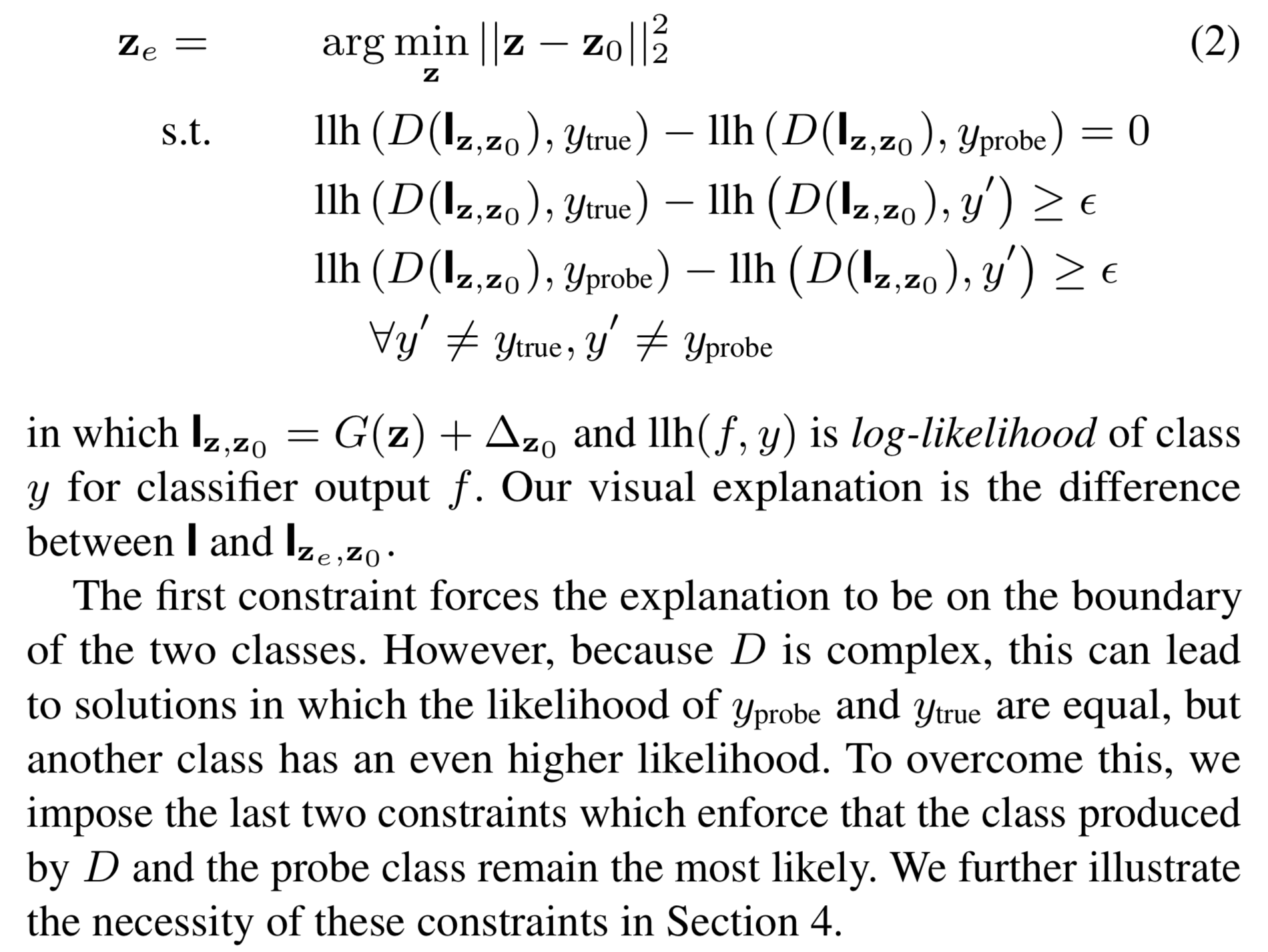
To find $z_e$:

After finding $z_e$ that minimizes L2 distance between $z$ and $z_0$, and that is in between the constraints, we compute the difference between $G(z_0) - G(z_e)$. This is done because we want to find a latent vector $z_e$ such that the resultant image has a similar style to the generated image from $z_0$, but is classified as our label of interest. By taking the difference between $G(z_0) - G(z_e)$, the overlapping parts are unchanged and parts that are different stands out.
Figure 3: An alternative way to the working the algorithm 1 and 2.
2.1. Another way to see it
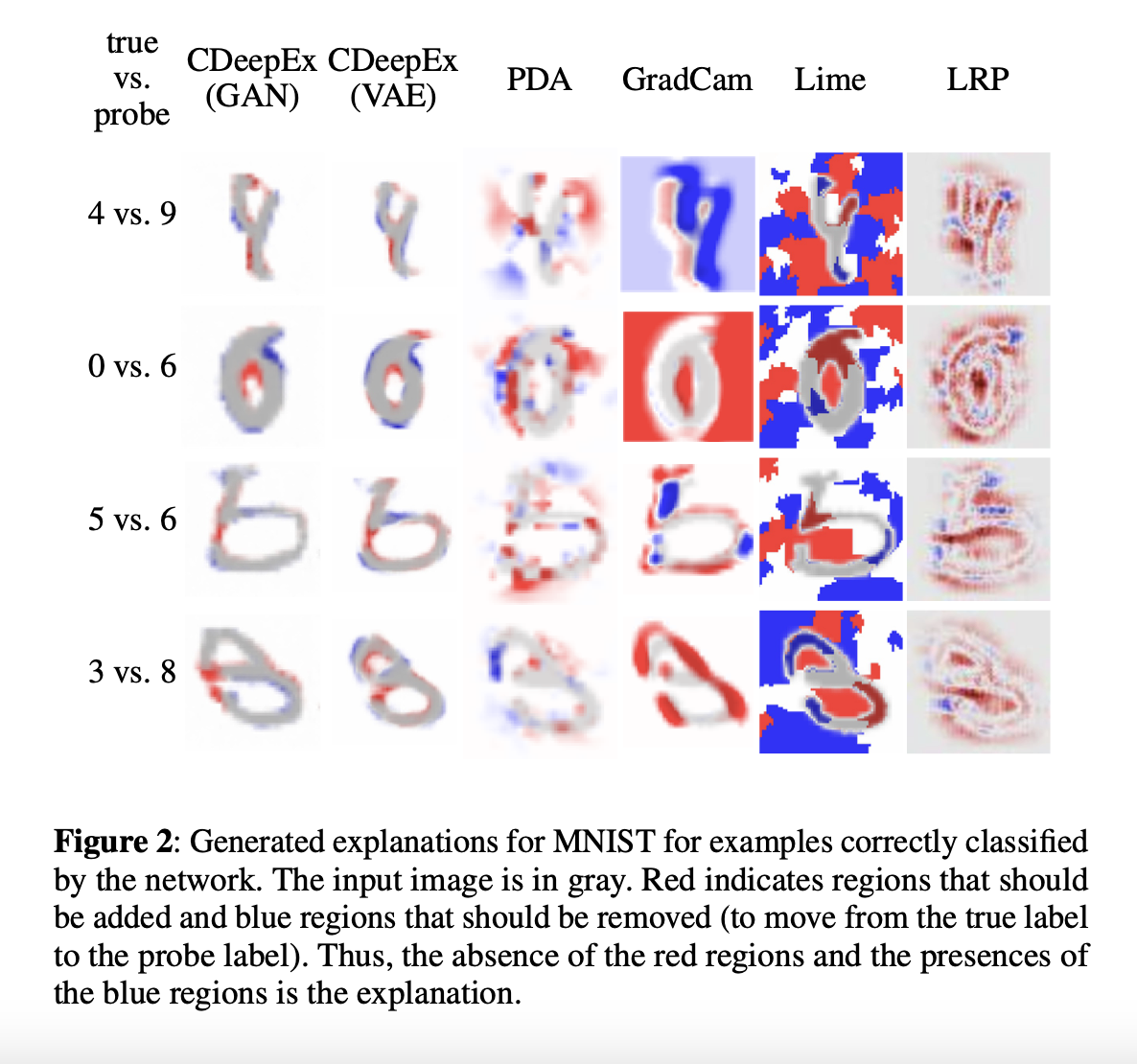
The suggested methods work well on the MNIST dataset, showing the transformation needed for Image A classified as the Number 8 to be classified as the Number 3. In the experiment is show different pair of number and the transformation need to be classified into different class.

Instead of representing the transformation as red or blue for regions that should be added or removed, the transformations are represented as a timeline that shows the sequence of transformation needed to covert Image 9 to converted into Image 3.
Figure 4: The framework to view the problem differently. (a) Use a VAE (Decoder) or WGAN (Generator) to generate images. Start with an image 9 from the MNIST dataset and update the latent vector $z$ to be close to this image, obtaining $z_0$. (b) The updated latent vector $z_0$ generates an image classified as class 9. We update the latent vector $z_0$ to get $z_e$ which, when generated, is predicted by the classifier as the class 3. During the process to update $z_0$ from Image 9 to Image 3, we got these sequence of transformations.
Figure 4: Part (a)
def learn_z0(G, I, lr, loss_fn, epochs, z0):
    # G is the generator
    # I is the image from a dataset
    # lr: Learning rate for the optimizer (default: 0.0005)
    # z0 the random initialized latent vector
    # set the optimizer "Adam" to optimize the loss with respect to the latent variable z0
    optimizer = optim.Adam([z0], lr=lr)

    # Iterate over epochs
    for _ in range(epochs):

        # set the calculation of the gradients for z0
        z0.requires_grad = True

        # generate the image from z0
        G_z0 = G(z0)

        # Calculate the loss (the loss is the norm l2 squared)
        loss = loss_fn(G_z0, I)

        # backpropagate the error and get the gradients
        loss.backward()

        # update z0
        optimizer.step()
    return z0,
Figure 4: Part (b)
def learn_ze(G, D, epochs, z, y, lr=5e-4, some_pixel_threshold=5):
    # G: Generator model
    # D: Discriminator model
    # epochs: Number of training iterations
    # z: Latent vector (input noise for the generator)
    # y: Target labels for the discriminator's output
    # lr: Learning rate for the optimizer (default: 0.0005)

    # some_pixel_threshold: Threshold for pixel difference to store generated images (default: 5)

    # Ensure the latent vector requires gradient computation
    z.requires_grad = True

    # Initialize the Adam optimizer to update the latent vector z
    optimizer = optim.Adam([z], lr=lr)

    # List to store generated images that meet the pixel difference criterion
    grid_images = []

    # Variable to store the previously generated image for comparison
    prev_stored_image = None

    # Training loop over the specified number of epochs
    for _ in range(epochs):
        # Generate an image from the latent vector z and pass it through the discriminator
        D_z, G_z_resize = discriminator_gen(G, D, z)

        # Compute the cross-entropy loss between the discriminator's output and the target labels
        loss = F.cross_entropy(D_z, y)

        # Backpropagate the loss to compute gradients
        loss.backward()

        # Update the latent vector z using the optimizer
        optimizer.step()

        # Check if there's a previously stored image to compare with
        if prev_stored_image is not None:
            # Calculate the pixel-wise difference between the current and previous images
            pixel_diff = torch.norm(G_z_resize - prev_stored_image).item()
            # If the difference exceeds the threshold, store the current image
            if pixel_diff > some_pixel_threshold:
                grid_images.append(G_z_resize[0].detach().cpu().permute(1, 2, 0))
                # Update the previous stored image to the current one
                prev_stored_image = G_z_resize.clone().detach()
        else:
            # If no previous image exists, store the current image
            grid_images.append(G_z_resize[0].detach().cpu().permute(1, 2, 0))
            # Set the previous stored image to the current one
            prev_stored_image = G_z_resize.clone().detach()

    # Return the optimized latent vector and the list of stored images
    return z, grid_images
I believe this view of the problem will be useful to understand how the network classifier goes through the latent space to find the image the outputs the correct label. Instead of depending on two variables to change an image A to an image B, is shown a sequence of transformation applied to image A to become image B.
3. Related Work
Several methods are made to interpret deep learning models. These methods can be segmented based on their approach to understanding model decisions:
3.1. Network Visualizers
This method has the goal to understand the knowledge of a network by looking at individual neuron or group of neurons. By analyzing each neuron in a network we want to find features, like edges or textures that influence the predictions of a network. However, is uncommon to find features that have a dedicated neuron to it, instead we analyze a group of neurons, which give a more understandable insight of a network.
3.2. Input Space Visualizers
Input space visualizers focus on explaining which parts of an image have the largest impact in a network decision. These methods are archived by modifying the input and observing how the output changes. Methods like xGEMs uses a GAN to find a contrastive example where tries to find a why not explication, however, in this method there is no formulation of a constrained optimization that give a more coherent explanation between Image A (original image) and Image B (Desired image).
3.3. Justification-Based Methods
These methods generates human-like like textual or visual to justify a network classification. While this methods give an easy way to understand a network decision, they do not always reflect the classification made by a network. Instead, it gives what humans expect to hear.
The main advantage of CDeepEx is that do not rely on of modifying the network or using heuristics. Instead, we use generative latent-space models, were by using the latent-space as a bridge between network understanding and human understanding we produce explanation in the form of natural-looking images.
4. Remarks
In the paper CDeepEx provides a method for generating contrastive explanation, which can be used to understand why a model predicts the class A over class B for the image A. Also in the paper is shown interesting results. This includes:
- A detail analysis on the MNIST dataset.
- The selection of the generator model, where is shown the impact in the performance with different datasets with respect of using a VAE or WGAN.
- An analysis of biased MNIST, were is tested if the method can provide clear explanations for a bias classifier.
- Also, this method is tested on the CelebA dataset (a dataset with celebrities faces) and Fashion MNIST, which shows how robust the method is for more complex datasets.
I encourage you to read the paper for more details.
Thanks for reading!
Cite as:
@article{
  tajia2024contrastive,
  title={Contrastive Deep Explanations},
  author={Tajia, Pedro},
  year={2024},
  howpublished={\url{https://pedrotajia.com/2024/11/24/Contrastive-Deep-Explanations.html}}
}
Reference
-
Feghahati, A., Shelton, C. R., Pazzani, M. J., & Tang, K. (2021). CDeepEx: Contrastive Deep Explanations. ECAI 2020. PDF
-
Gulrajani, I., Ahmed, F., Arjovsky, M., Dumoulin, V., & Courville, A. (2017). Improved training of wasserstein GANs. ICML, 30, 5769–5779. PDF
-
Kingma, D. P., & Welling, M. (2014). Auto-Encoding Variational Bayes. ICLR. PDF